Jim Lovell is a landscape photographer based in Hobart, Tasmania. Jim's recent work has been focused on capturing the essential elements of the Tasmanian landscape using long exposure techniques.
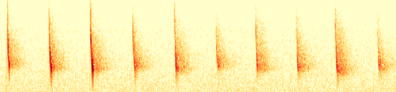
We recently took a trip to the east coast of Tassie for the summer holidays. Something I was keen to do was to try out the MarkII at low frequencies by searching for Bitterns, so one evening I put out the MarkII at Moulting Lagoon together with an AudioMoth recorder. No luck with the Bitterns but there were plenty of bats and I was able to get some nice tracks. Here’s one that turned out really well:
I still have some work to do to improve the direction-finding algorithm and I think I can improve the calibration too. Things are pretty reliable when the bat calls span a good frequency range but narrow-band signals are a little more challenging. I’m also experimenting with different microphone configurations, which may help here too.
The Batto Mark-III?
I’m beginning to think about a MarkIII recorder that would have 6 microphones and provide distance as well as direction, for bats at least. The Teensy 4.1 looks like a good candidate for the controller board as it can support that number of mics (or more).
I’ve been spending the past few weeks working with more data and trying to make the direction finding software work more efficiently and be a little more automatic and reliable.
Bat calls that cover a wide frequency range are generally easier to locate than the narrow-band calls. (This makes sense as the slope in phase across the band gives an unambiguous delay estimate if it covers enough frequencies, but doesn’t do so well for narrow coverage). So some data are hard to interpret and there have been some fly-bys I haven’t been able to track. This could be improved by a better arrangement of microphones I think.
Here’s a screenshot of some software I built to help with localising the signals and resolving ambiguities. For every chirp I calculate the coherent average of the signal strength and find directions on the sky where this is a maximum, In many cases there are multiple maxima of similar amplitude so I’ve been using The SciPy optimisation routines to find local maxima across the sky. The top panel is the spectrogram, below that is amplitude vs time for the 5 strongest maxima (the darker the red, the greater the amplitude). The next panel is a plot of possible azimuth solutions vs time, then elevation below that. Finally, the two plots at the bottom show sky distribution in two different projections. Usually I can use the brightest signals to ‘anchor’ the remaining chirps and find the trajectory. But you can see the ambiguities, and I need to work on that. The movie shows the final processed result.
It’s been a year since I last posted! Where did the time go?
The MarkII has had a few changes over the year. I’ve moved to three D batteries for the main power supply, which gives a couple of nights continuous recording, and I’ve improved the wiring which has stabilised things a lot. The microphone array is now on the end of a ~1m cable and the electronic interference I was picking up in the data has pretty much gone. I’ve also started on coming up with a suitable enclosure for the microphones that lets ultrasound in but doesn’t cause unwanted reflections. Still some way to go there, so for now I’m waiting for good weather and recording without any covering.
The main issue this year though has been the data. The problem I found with the phase breaking up past the leading edge of a chirp is present in the MarkII and I’ve also seen it in stereo data from Wildlife Acoustics SM2 recorders. In order to get a good phase measurement and therefore a direction, I’ve written some algorithms to just pick out the leading edge. These work reasonably well, but I’m finding at the moment that inspection of individual chirps is needed in order to fine tune things and get the right delay.
Data fitting and inspection software for localising the audio signals. The left-hand panels show amplitude vs frequency on the top with phase vs frequency for each baseline below. The map in the top right is an all-sky map with the colours indicating how well the data phase matches a sky position.
Anyway, the good news is that I am able to measure directions with the MarkII! Here’s a graph showing a call recorded in my garden last month. The spectrogram is at the top, and below is a sky map showing the path that the bat took (Imagine you’re lying on your back with your head pointing north. The sky map shows the path the sound took, each point is an azimuth and elevation measured from the chirp). The bat mooched around near the neighbour’s fence to the east, flew west and took a right almost over the recorder, then headed off to the north.
Spectrogram (top) and sky map showing a bat flight through the back garden.
So some really good progress at last! The next steps are to improve the processing algorithm and hopefully automate the position analysis, re-arrange the microphones into a configuration that provides better positions (i.e. play with the separations and orientations of the mics), find a good weather protection solution, and do some more field tests! At some stage I’d like to change to microphones that work better at ultrasonic frequencies, for more sensitivity and so I can push the sample rate up to 384 kHz.
With only a pair of microphones, there isn’t enough information to fully track the trajectory of the bat. You can only get the angle orthogonal to the baseline as a function of time. However, if we make a few assumptions, it’s possible to model data and get some idea of what the bat was doing. So, if we assume that the bat was travelling in a straight line at a constant speed, we can find a starting position and velocity that agrees with the data. After a little playing around with some geometry and a python script, here’s what I came up with. The graph shows the data I reported yesterday (angle vs time) and the model trajectory:
A model for the bat’s flight across our back garden. Data in orange and the model in blue. Starting positions and the velocity components in x, y and z are shown.
While it’s probably not a unique solution and not very well constrained, the data are consistent with a bat moving at 5 m/s at a height of 4.4m, which doesn’t sound too unreasonable.
Last time I showed some results from test data aimed at finding out how well directions can be determined using the cross-correlation technique. I’m now going to look at some real data and see how well it does, and for that I’m using a couple of observations made back in January. The first is of a wattle bird and the second is a bat.
Bird data
So firstly, here’s the bird: a little wattlebird (Anthochaera chrysoptera). It’s a pretty noisy one and had a broad audio spectrum, so is a nice test case. At the time of recording, the bird was just sitting in a tree and not moving. Here’s a plot that summarises the data:
A little wattlebird (Anthochaera chrysoptera), observed on 10 Jan 2019. The main panel shows the spectrogram and the white vectors are the measurements of direction to the signal (vector length is related to signal strength). The top two panels show signal strength (measured in signal-to-noise ratio) and direction as a function of time for the frequency of the loudest signal (2.9 kHz, indicated by the horizontal line). The two right panels show SNR and direction as a function of frequency (indicated by the vertical line) at the time of the peak.
The direction measurements all look good and consistent across the frequency range. This is pretty surprising given that the baseline is only 15mm which is 13% of a wavelength at 2.9 kHz (118 mm). The ability to measure position is related to signal strength, so here’s a plot that shows that behaviour for the bird data:
Sensitivity to direction as a function of signal strength for the little wattlebird observation.
The above plot shows that the scatter in direction measurements decreases with increasing signal strength as expected. Even at such a short baseline compared to the wavelength, it’s possible to get angles to about 20 degrees at 3-sigma for strong signals.
Bat data
Next is a bat observation which was a little more challenging to process given the higher frequency and the issue of resolving phase turn ambiguities. Fortunately this wasn’t a problem in this case. Here’s what the data look like after processing:
A long-eared bat (Nyctophilus spp) (I think!) observed on 23 Jan 2019. The main panel shows the spectrogram and the white vectors are the measurements of direction to the signal (vector length is related to signal strength). The top two panels show signal strength (measured in signal-to-noise ratio) and direction as a function of time at 38 kHz (indicated by the horizontal line). The two right panels show SNR and direction as a function of frequency (indicated by the vertical line) at the time of the peak. Note the clear change in direction as the bat flies past!
This is pretty exciting I reckon! The phases clearly show the bat moving from left to right with the angle changing by about 60 degrees over 7 seconds. It looks as though the systematics kick in in delay at about the 10 us peak-to-peak level which at this frequency and a 15mm baseline corresponds to 10 degrees in direction:
Amplitude, phase and delay against frequency for a 0.02 sec sample.
So far I've been looking at signal strength but there's another fundamental quantity that an interferometer measures: phase. Amplitude tells you how bright (loud) something is but phase tells you the direction it's coming from. How well does the prototype detector do this?
As promised here are some observational data that show the improvement in signal-to-nose with a cross-correlation. Here’s a spectrogram of the bird call:
In radio astronomy the signals being collected are typically much weaker than the noise and a lot of effort is put into building high sensitivity, stable receiving systems. The individual telescopes are big to collect as much light as possible and hence reduce integration times. One method that can improve signal-to-noise is interferometry, where signals from two or more telescopes are cross-correlated (in pairs). The signal from an astronomical source, received by each telescope will be preserved but the noise that is different at each telescope will be different and therefore suppressed in the correlation.
The following simulations are of audio data with similar properties to my data from the prototype recorder. Sampling is at 96 kHz giving a maximum audio frequency of 48 kHz. The initial assumption is that the microphones are co-located and therefore there is no delay between receiving the same signal.
Background noise
These simulations compare the noise levels from a single microphone to that obtained by combining two of them. The data are combined in two ways:
The first is a simple summation of the data streams in the time domain. This emulates a technique that is commonly used in the data collection process. Adding the two signals together doubles the signal strength (i.e. a 6 dB increase) and increses the noise by 3 dB for a 3 dB improvement in SNR overall (InvenSense Application note AN-1140).
A technique used for radio interferometry is to cross-correlate the two data streams. This is done by multiplying the Fourier transform of one channel by the conjugate of the Fourier transform of the other.
The noise that is recorded from each microphone will contain a component generated by the microphone itself as well as noise generated elsewhere in the system that is common to both.
In this simulation two data streams are made that contain only random Gaussian noise with a fraction of that noise common to both that is varied. If all noise is common then there should be no difference between the single and two-microphone case. The signal noise floor has been calculated as a function of this fraction.
The following plot shows the predicted noise floor for a single microphone ("Left"), the sum from a pair of microphones and the cross-correlation of the two signals. As predicted, in the case where the noise from the two microphones is independant (i.e. fraction correlated noise is zero), the noise floor for the sum of two data streams is a factor of two (3 dB) higher. A cross correlation shows dramatic improvement in noise level. For example, data where 10% of the noise is common to both channels will result in a 10 dB decrease in noise.
Simulated noise floor as a function of the fraction of noise common to both signals.
We can compare these predictions with actual data from the prototype recorder. For this test, I wanted to measure the noise floor so the microphone pair was sandwiched between two pieces of acoustic foam[^1] and a two-second recording was made.
The following graph shows the power spectral density as a function of frequency for the two microphones, their sum and the cross-correlation. Unlike the simulated data, which assumes that noise is constant as a funtion of frequency, the microphones have a changing response across the band.
The spectral density plot shows very similar noise floors within the specified range but significant differences above that. It is however very clear that the noise floor of the cross-correlated data is much lower than the individual microphone signals.
[^1]: Which we originally bought to attenuate the sound coming from my son's drum kit!
The noise floor for two microphones, their sum and cross-correlation
The next graph shown the difference in power levels of the summed and cross-correlated data as a function of frequency. For the range of frequencies below 15 kHz, the 3 dB change is clearly seen. The improvement in noise for cross-correlated data is approximately 10 to 15 dB with an average of ~-12.5 dB or a factor of 0.056 or 6% correlated noise. In other words, over 90% of the internal noise can be removed using cross-correlation.
Comparison of noise floors on individual microphones with summed and crossed-correlated signals.
Signal to noise ratio
In the next set of simulations I combined the noisy data with a 10% common component with an input signal to estimate the difference in signal-to-noise betwen single and dual microphone configurations. The expectation is that the cross-correlation technique will provide the ability to detect much weaker signals than a single microphone or the sum of signals from two microphones.
A 15 kHz signal was inserted at varying intensity. The peak value was measured and compared to the noise level. To make the comparison clearer, the summed data have been expressed as an average (i.e. (Left+Right)/2). The following figure shows measured signal strength compared to input. As the signal gets weaker, the measured signal at 15 kHz becomes more and more dominated by the noise and the curve departs the input=output line. As expected, the average and cross correlation techniques perform better than a single microphone with the cross-correlated data the most sensitive.
The next plot shows signal-to-noise ratio (SNR) as a function of input signal strength and indicates the improvement in performance. If for example, the minimum acceptable SNR is 5, the minimum signal strength is
58 V/sqrt(Hz) for single mic
43 V/sqrt(Hz)for summed data
18 V/sqrt(Hz) for cross-correlated data.
In other words, for a SNR detection limit of 5, cross-correlated data is capable of detecting signals 3 times weaker than a single microphone and 2.4 times weaker than summed data.
Signal to noise ratio (SNR) as a function of simulated input signal strength
In the next post I’ll show some real signal detections and see if SNR is improved as expected…
Acoustic detectors are widely used for the non-intrusive study of wildlife. It turns out that the data collected by these detectors have some similarities to radio astronomy data, which I’m much more familiar with. I’m interested to see how applicable some of the astronomical observation and analysis techniques are and if they can be used in eco-acoustics. This blog describes my work to build a detector to collect and analyse audio data to try out some of these techniques as a proof of concept. I’m focusing on the use of multiple microphones (two initially) and cross-correlation of their signals to improve sensitivity and signal to noise as well as provide estimates of signal location and speed. Audio data at frequencies up 48 kHz are being recorded at present but the techniques will also work at higher frequencies..
The detector is based on a Raspberry Pi computer with a pair of digital microphones attached. The cost of components is relatively small, ~$100, making it a nice entry-level device for anyone who doesn’t mind wielding a soldering iron.
In the next post I’ll describe some work on using two microphones to improve sensitivity and show some initial results. Following that, I’ll look into methods to measure location and movement of signals.
The Batto Mk-I. A Raspberry Pi Zero, a pair of MEMS microphones, a battery, some buttons, LEDs and an e-paper display.